import numpy as np
import matplotlib.pyplot as pltEuler’s Method example
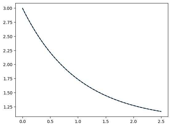
Use the differential equation below to find \(y\) when \(t=2.5\):
\(y(t) = 1 - \frac{dy}{dt},\quad y(0) = 3\)
Use \(\Delta t = 0.5\)
Solution
Let’s rearrange the differential equation so we have a “function for the derivative”:
\(\frac{dy}{dt} = 1 - y(t)\)
$ y(0) = 3$
\(\Delta t = 0.5\)
The analytical solution:
\(y(t) = 1 + (y_0 - 1) e^{-t}\)
# Define the derivative as a function of y, t
def dydt(y):
    return 1 - y

# Define Eyler's solution for the "next" value of y
def euler(dydt, yn, dt):
    ynp1 = yn + dt * dydt(yn)
    return ynp1

# Set our step size
dt = 0.0005

# Set our initial conditions
t = [0.0]
y = [3.0]

# Set the stopping point
stop = 2.5

while t[-1] < 2.5:
    # define the "current" condition
    yn = y[-1]
    tn = t[-1]

    # use Euler's method to get the next value of y
    yn_plus_1 = euler(dydt, yn, dt)

    # also increment t (for plotting and loop control)
    tn_plus_1 = tn + dt

    # add these new points to the lists of y and t
    t.append(tn_plus_1)
    y.append(yn_plus_1)

# For plotting reference, the analytical solution and a time array
def analytical(t, y0):
    return 1 + (y0 - 1) * np.exp(-t)

t_arr = np.linspace(0,t[-1])

plt.plot(t_arr, analytical(t_arr,y[0]))
plt.plot(t,y, "--", c="k")
# plt.scatter(t, y,marker=".",c="k")
plt.show()