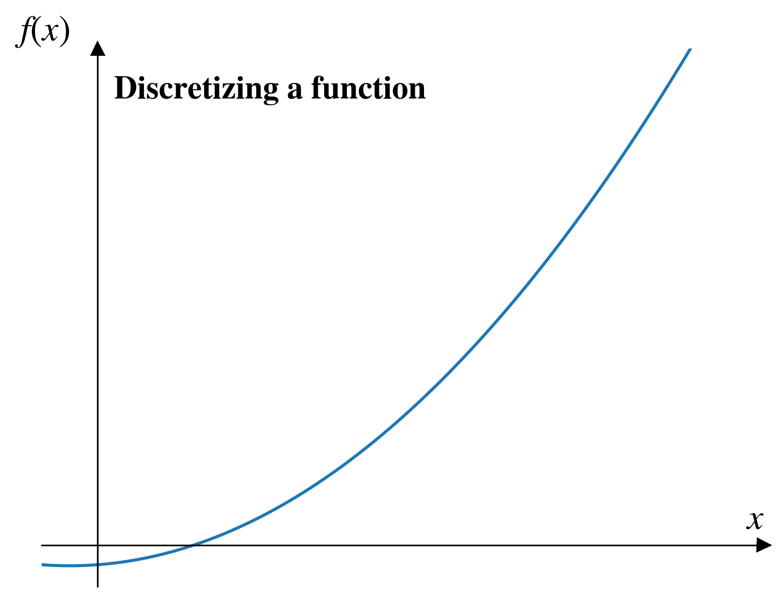
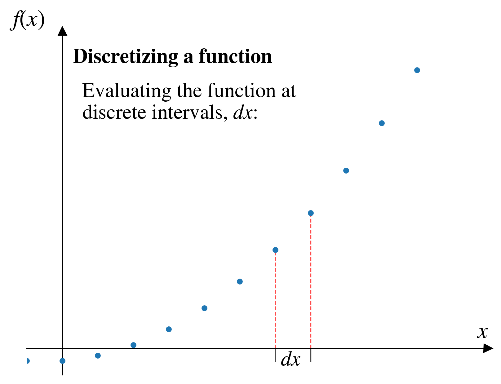
If we evaluate a function at intervals spaced at \(dx\), we are essentially converting our continuous function into a set of discrete data points.
From smooth to discrete
An example
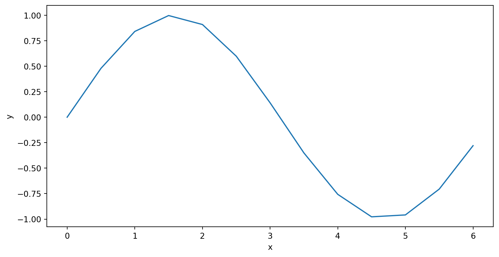
We discretize functions every time we plot them
dx =0.5x = np.arange(0,2*np.pi,dx)y = np.sin(x)
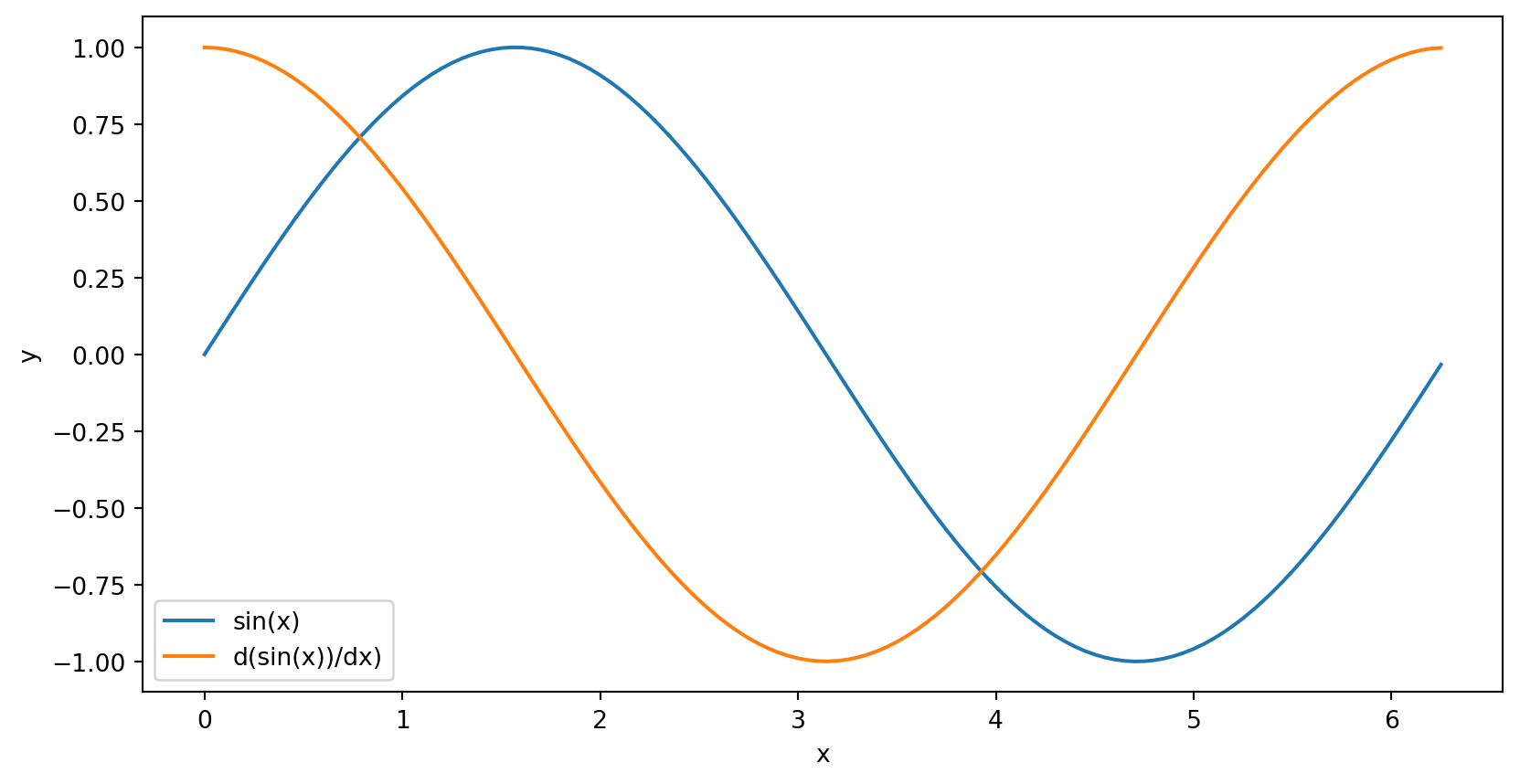
An example
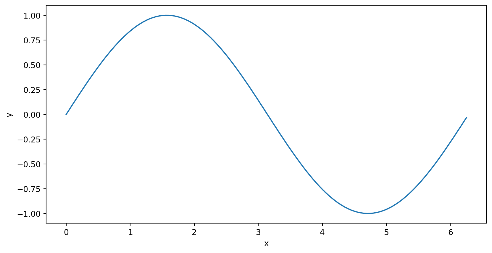
We discretize functions every time we plot them
dx =0.05x = np.arange(0,2*np.pi,dx)y = np.sin(x)
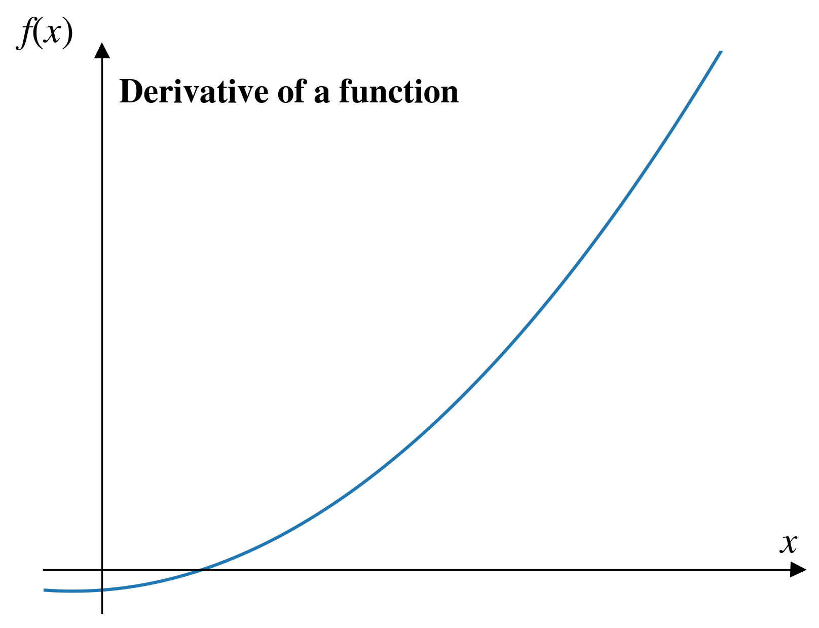
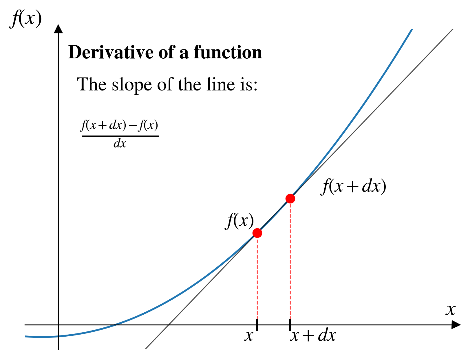
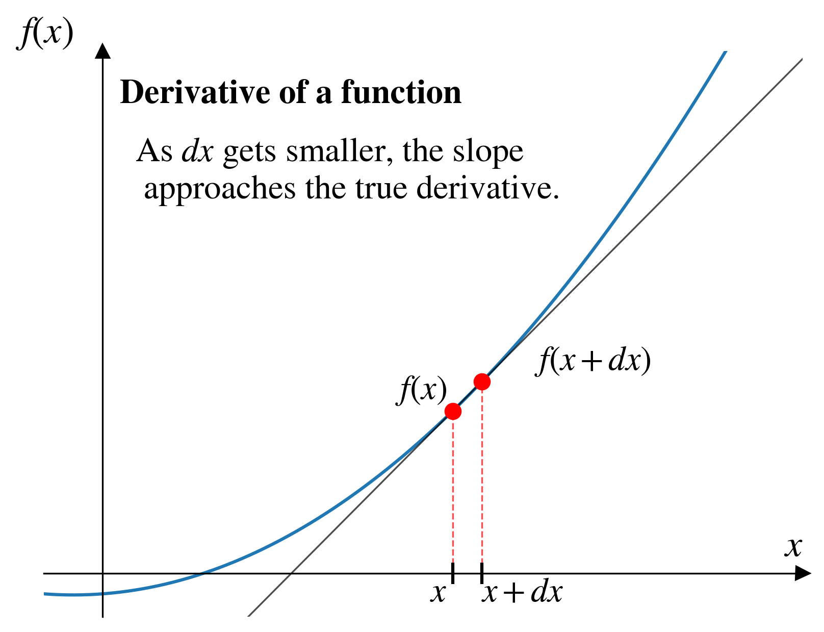
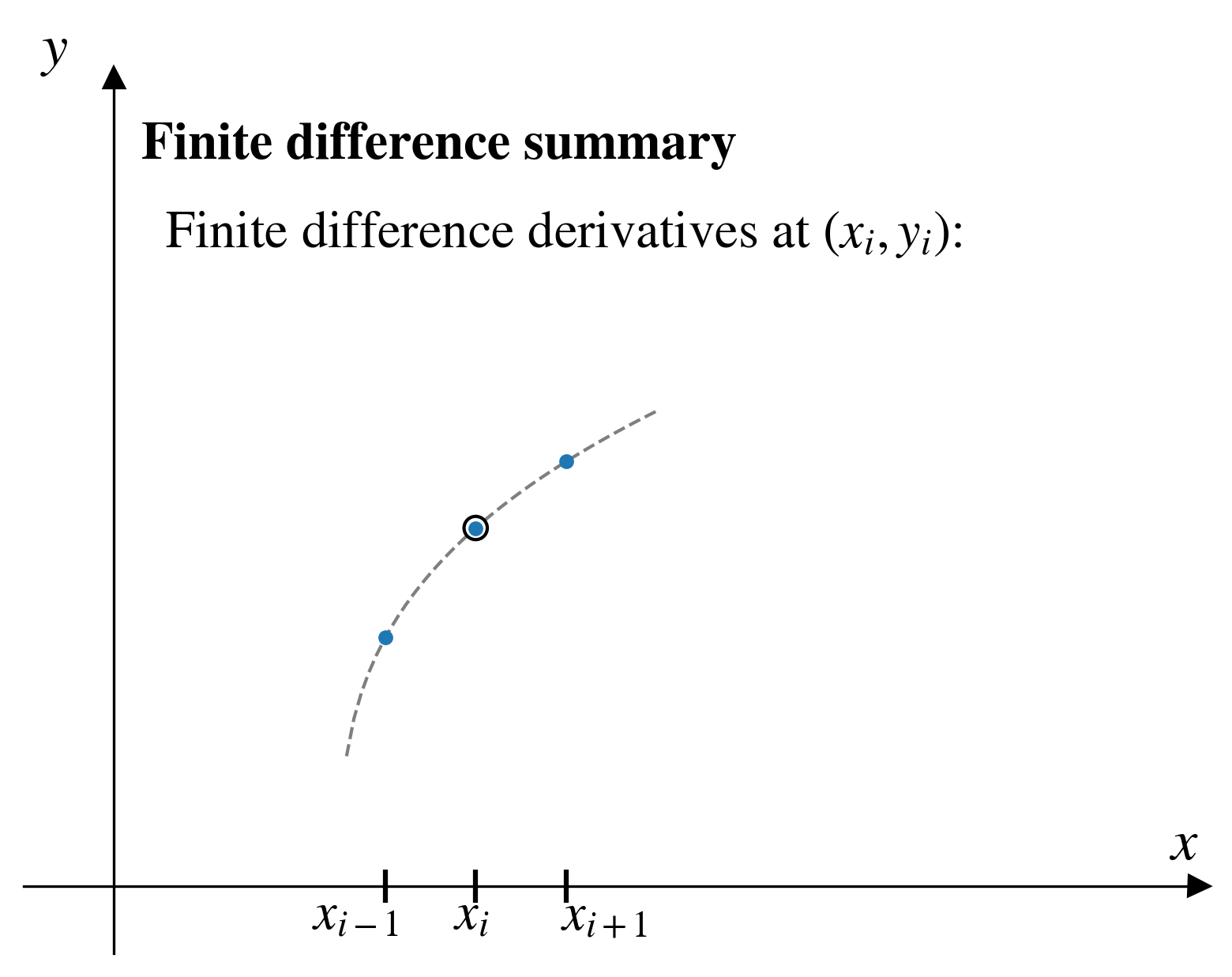
Numerical derivatives
Let’s apply these concepts to finding numerical derivatives using three simple approaches:
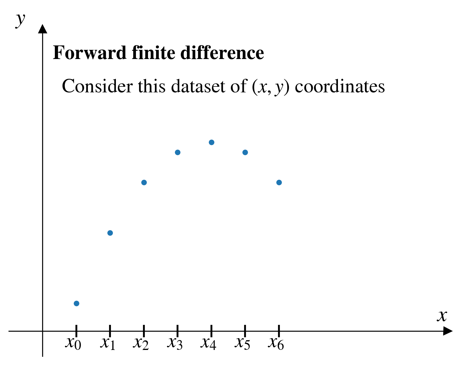
Forward finite difference (FFD)
Central finite difference (CFD)
Backward finite difference (BFD)
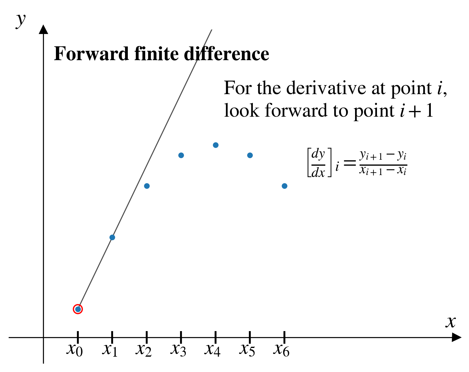
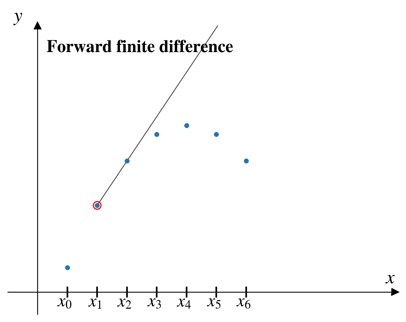
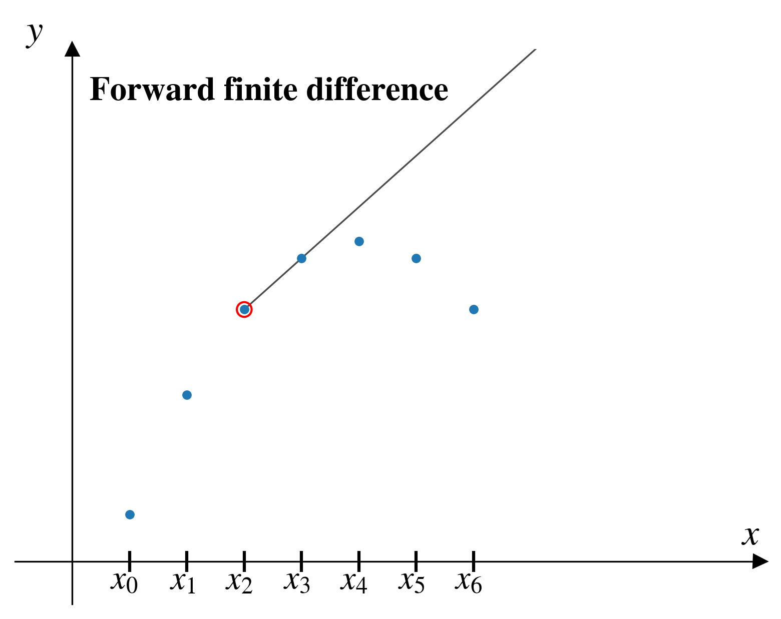
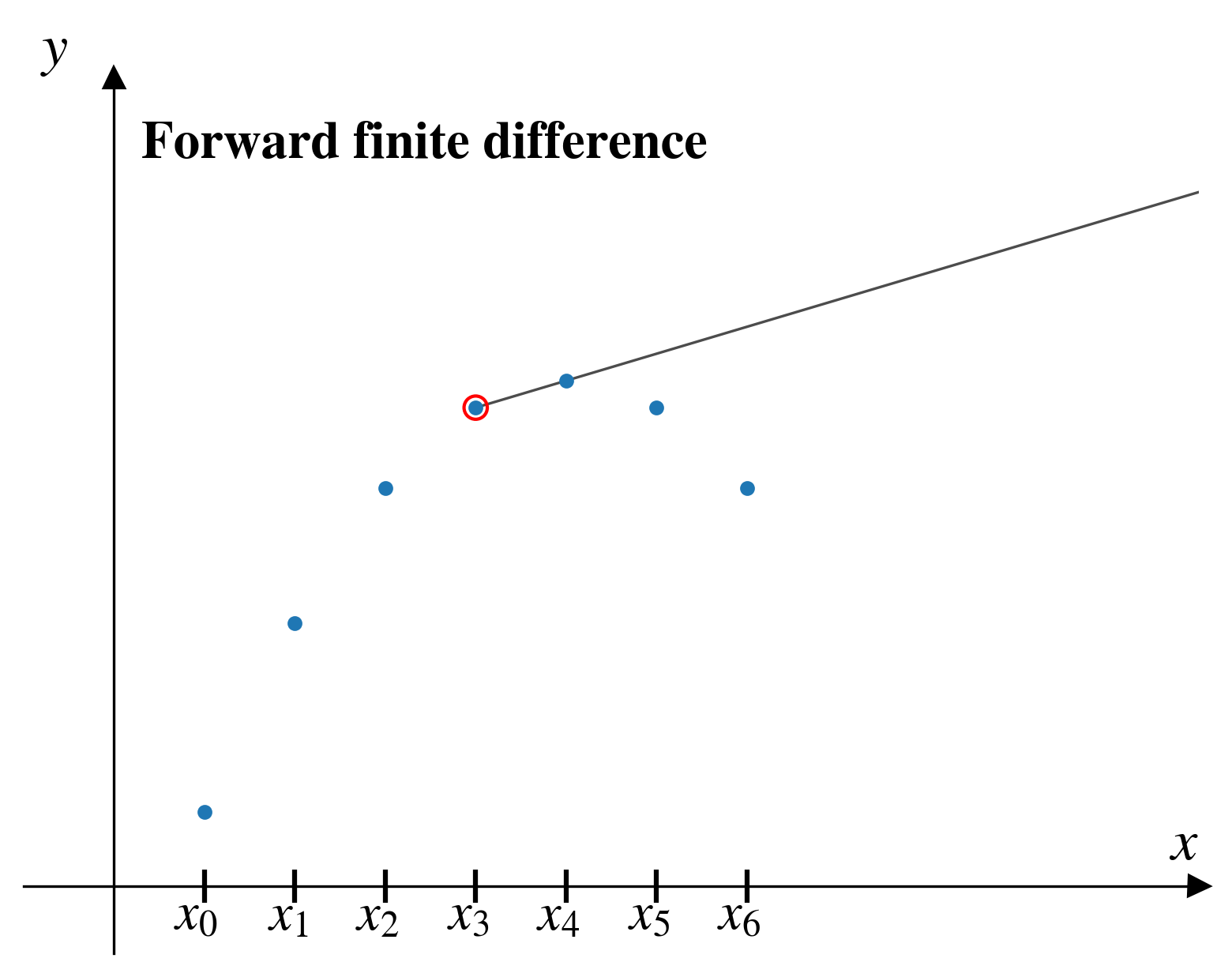
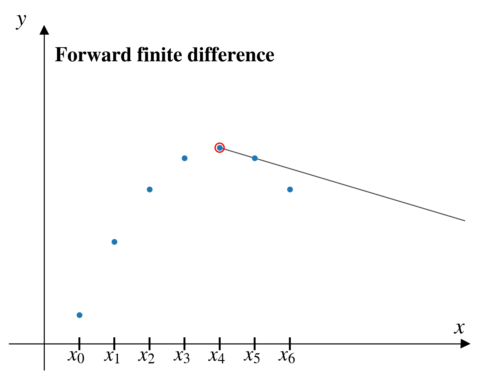
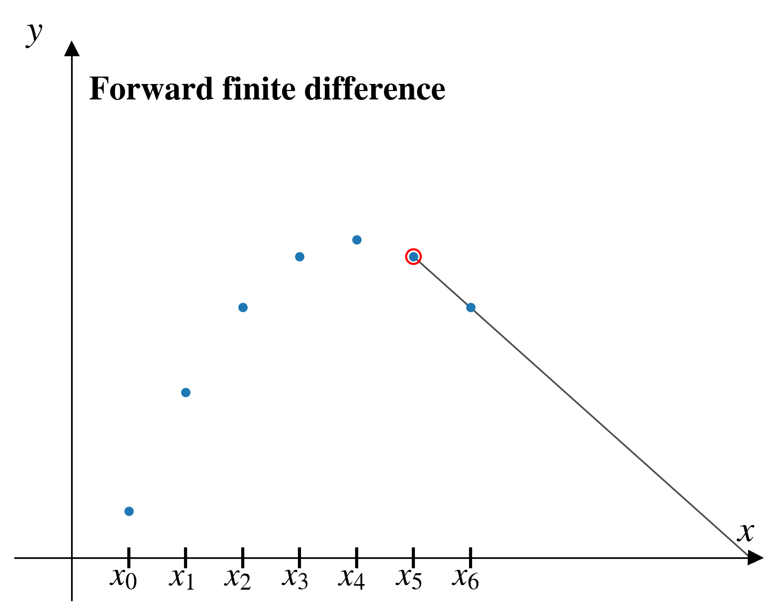
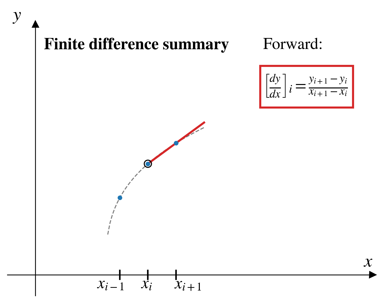
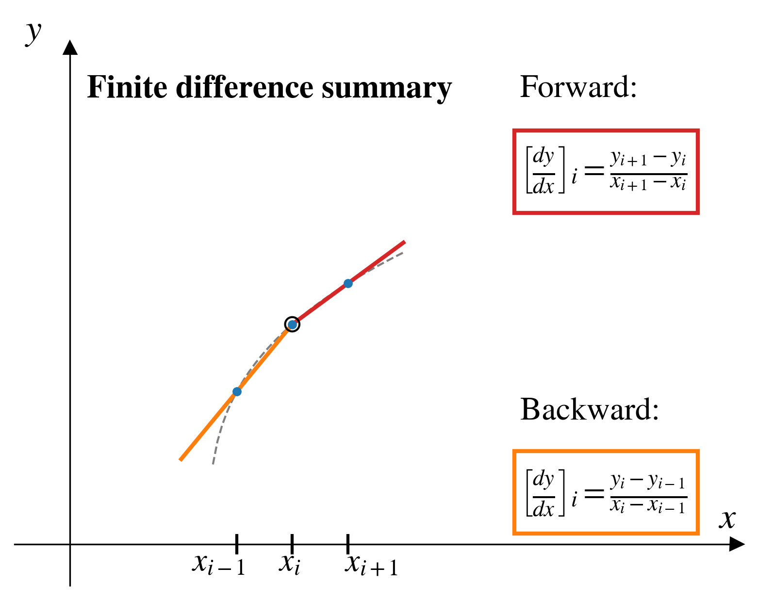
Forward finite difference
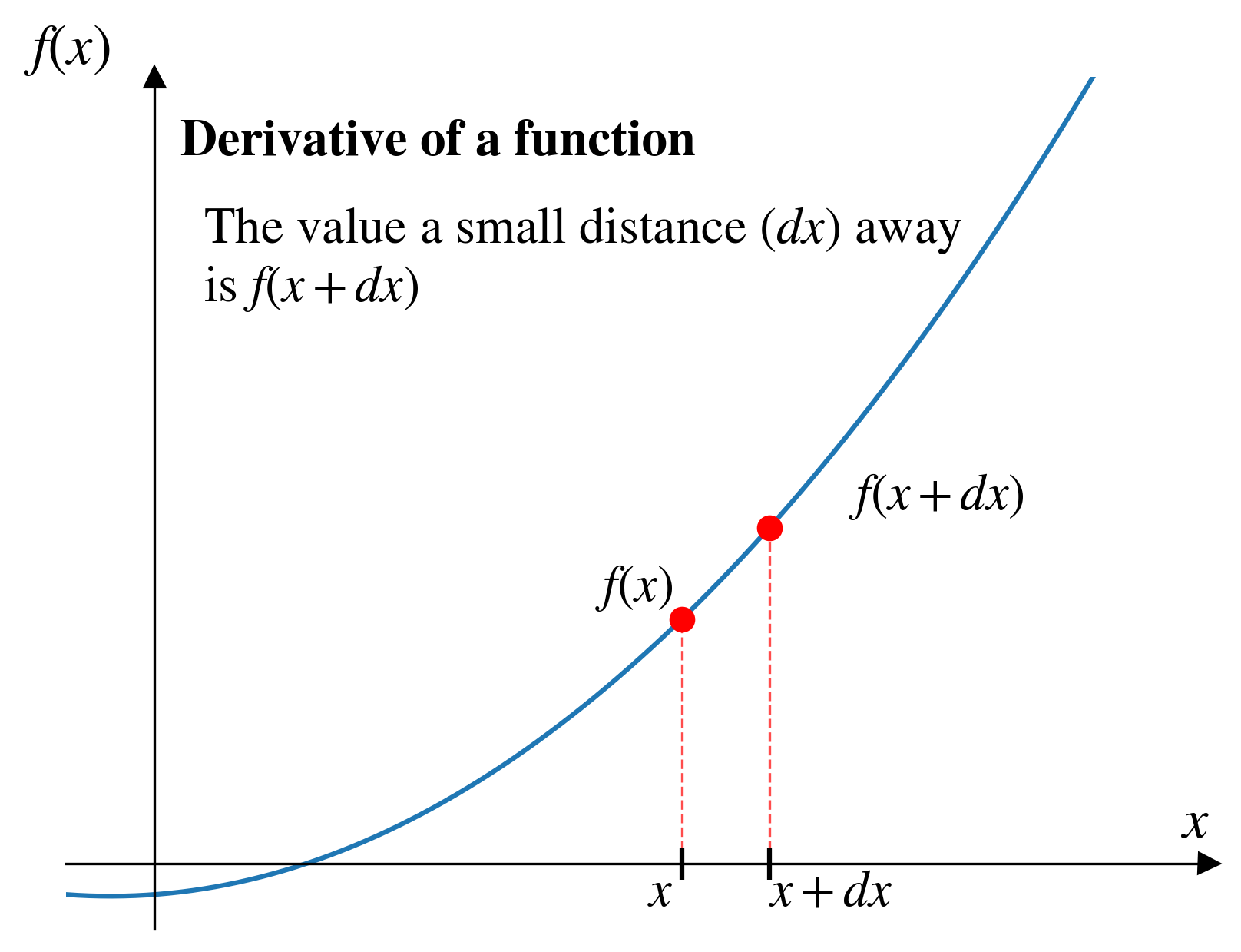
In the forward finite difference (FFD) method, from a given pair of points, \((x_i,y_i)\), we approximate the derivative by looking “forward” to the next pair of points, \((x_{i+1},y_{i+1})\)
As we step through the FFD, two problems are apparent:
We can’t estimate the derivative for our last data point!
For a dataset with \(n\) points, FFD will give us \(n-1\) estimates of the derivative.
The estimate seems inaccurate in several places.
Let’s address issue 2 first
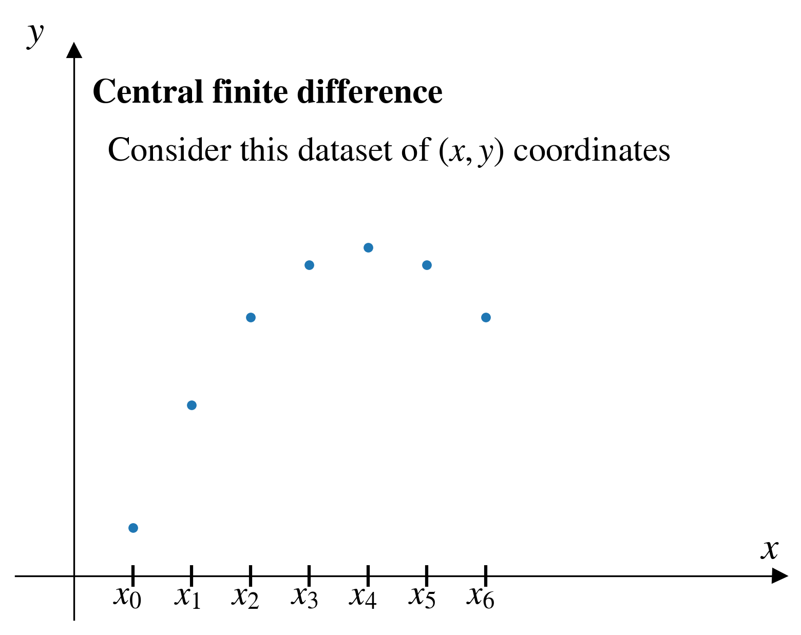
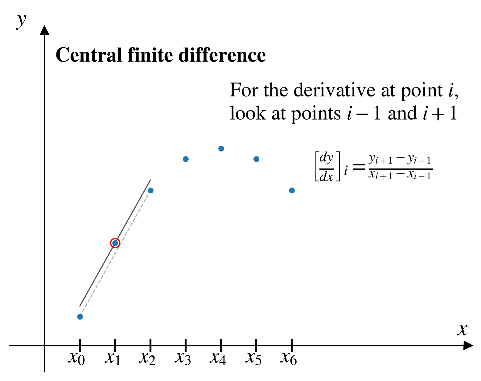
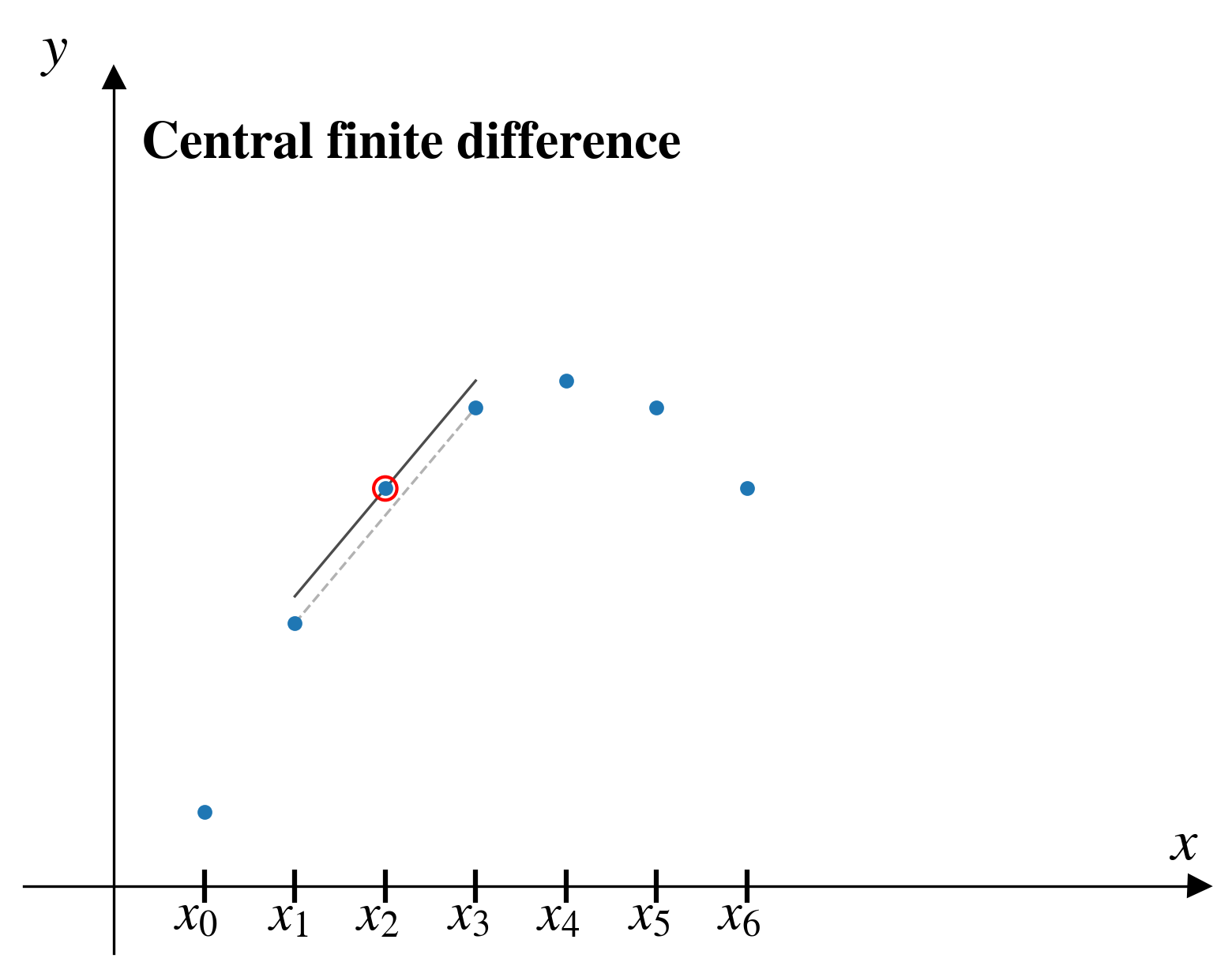
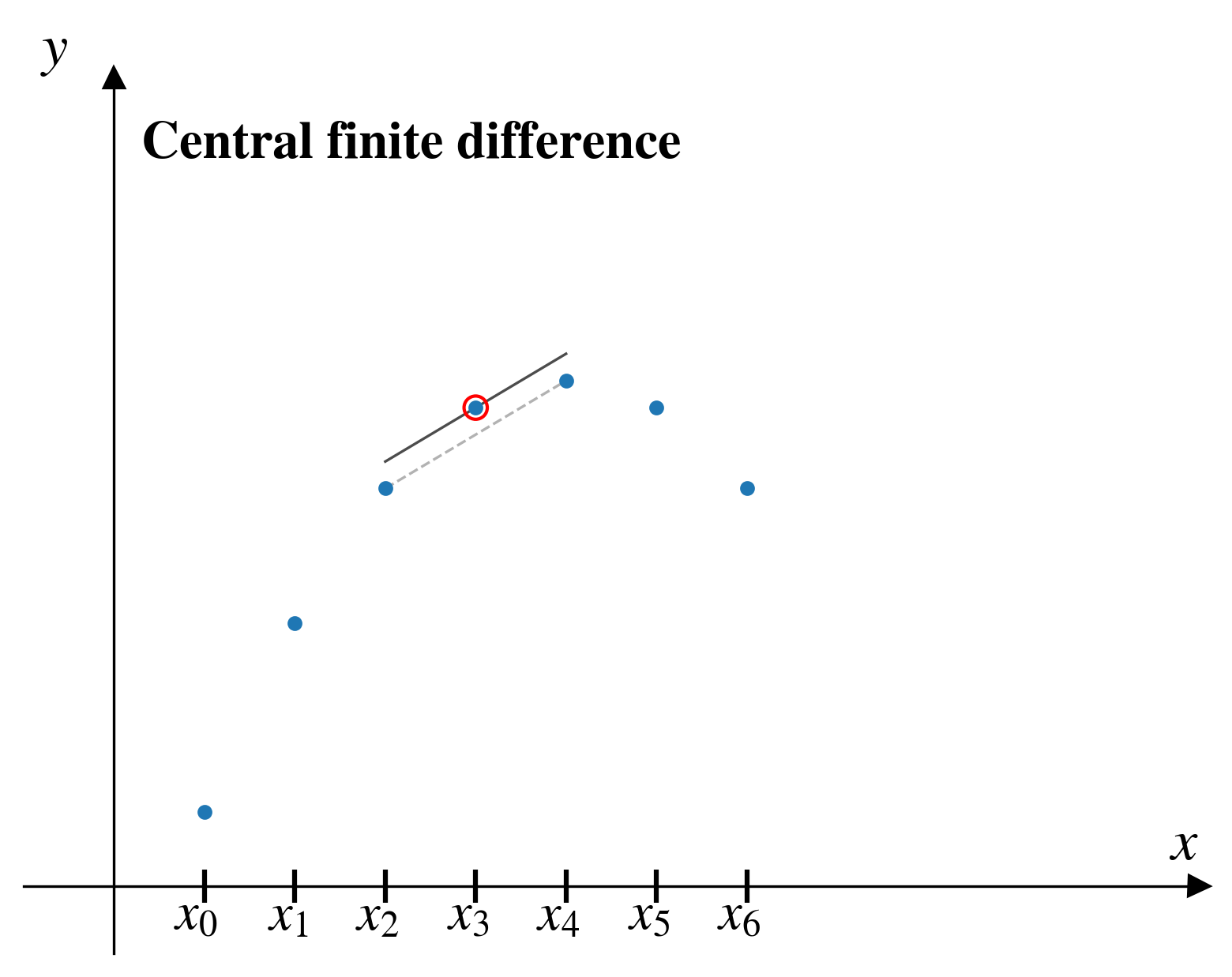
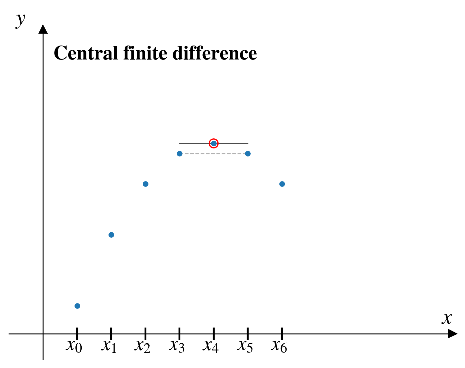
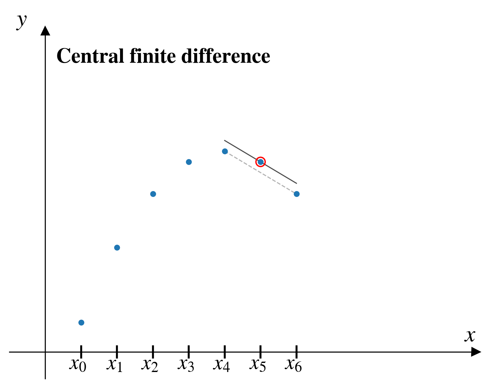
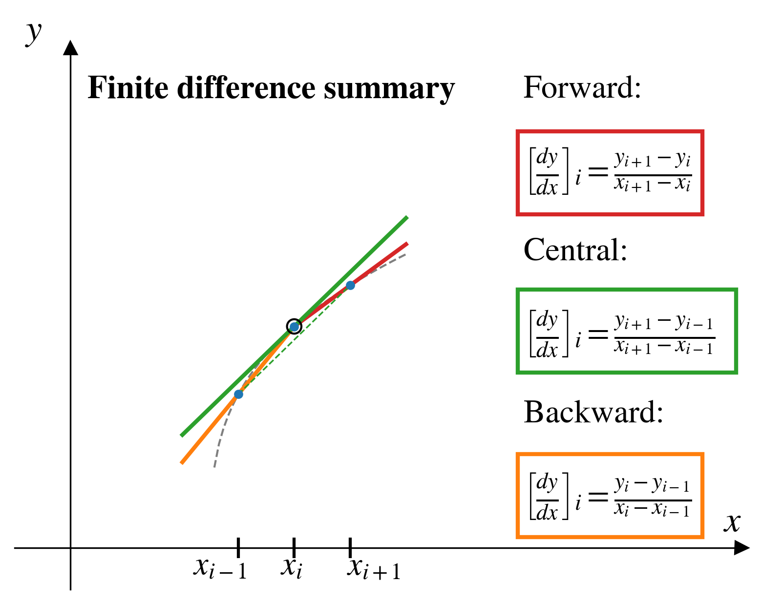
Central finite difference
In the central finite difference (CFD) method, from a given pair of points, \((x_i,y_i)\), we approximate the derivative by looking at the two pairs of points on either side: \((x_{i-1},y_{i-1})\)and\((x_{i+1},y_{i+1})\)
consider effect of data on both sides of the point of interest
But it has an even more limited range than the forward finite difference method:
For a dataset with \(n\) points, CFD will give us \(n-2\) estimates of the derivative.
Solution: use CFD wherever possible, use FFD when needed
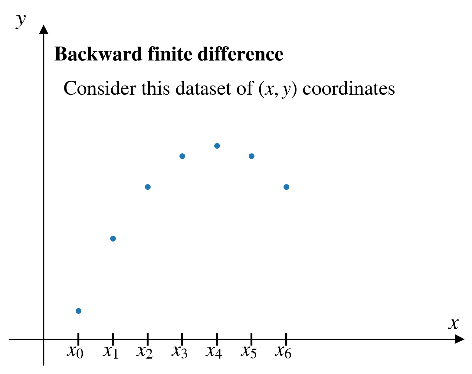
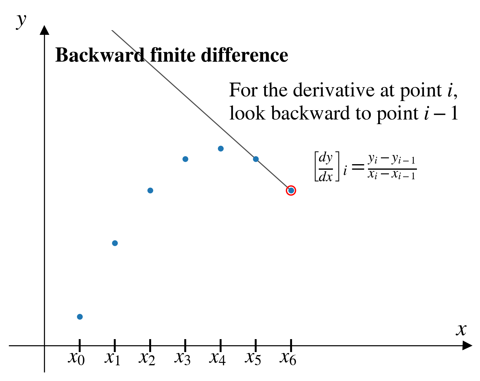
Backward finite difference
That still leaves us with \(n-1\) estimates…
Enter the backward finite difference method
In the backward finite difference (BFD) method, from a given pair of points, \((x_i,y_i)\), we approximate the derivative by looking “backward” at the previous pair of points, \((x_{i-1},y_{i-1})\)