TME 310 - Computational Physical Modeling

Euler’s Method for ODEs

Lorne Arnold, PhD, PE

University of Washington Tacoma

What is a differential equation?

Differential equation

an equation that relates an unknown function to its own derivative.

For example

\[y(t) = 3t + \frac{dy}{dt}\]

Analytical solutions

We’ve seen analytical solutions to differential equations.

For example, in the parachute problem, we used the solution to this differential equation: \[\frac{dv}{dt} = g -\frac{c}{m}v\]

which was:

\[ v(t) = \frac{gm}{c}(1 - e^{-ct/m})\]

Numerical solutions

But many differential equations don’t have closed-form (i.e., analytical) solutions.

For those, we need numerical methods to approximate solutions.

Euler’s Method

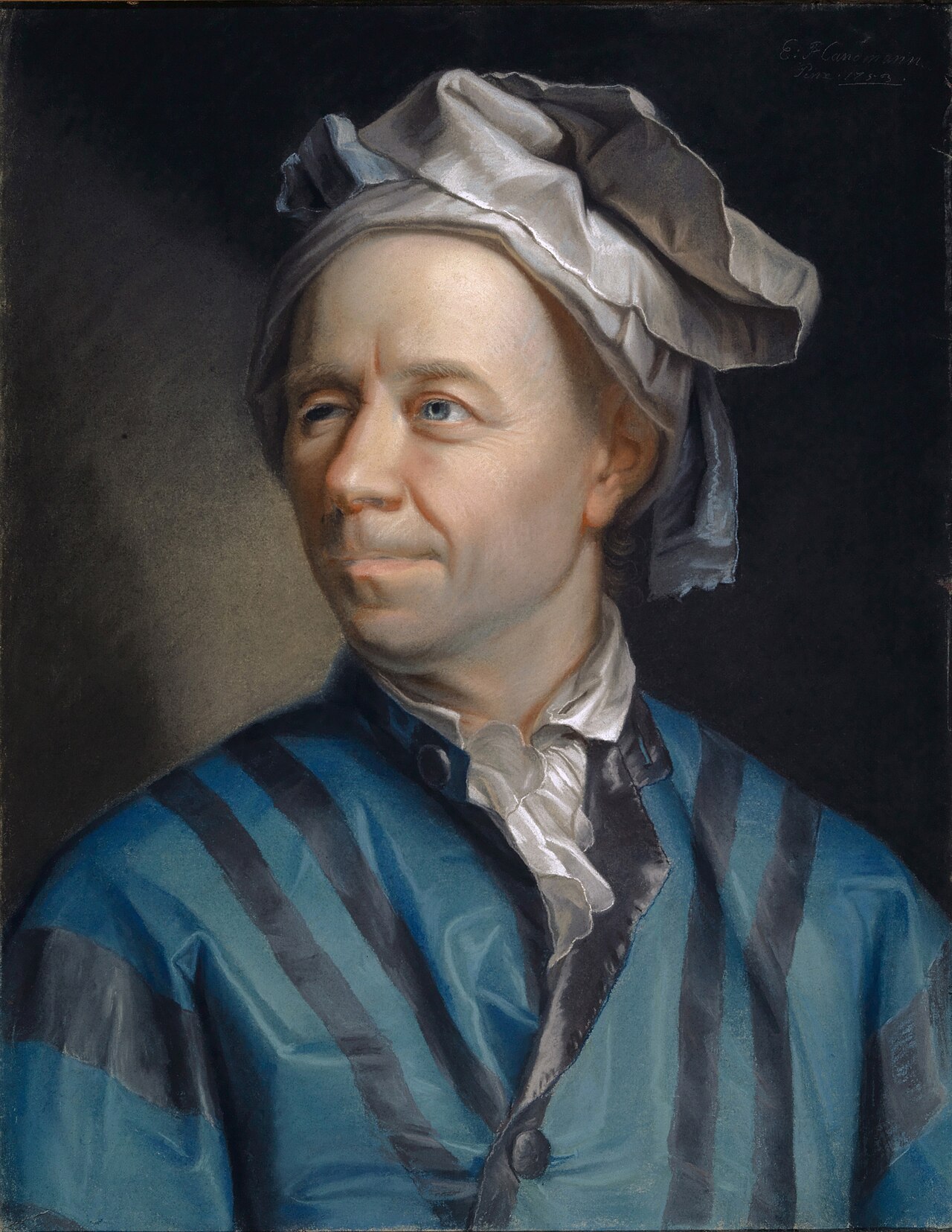
(1760’s) Euler developed a method that approximates the solution to a differential equation.
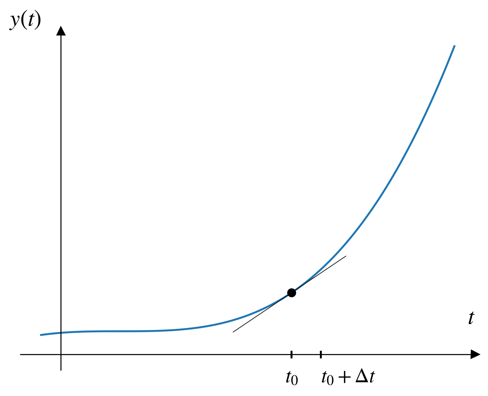
He realized that if

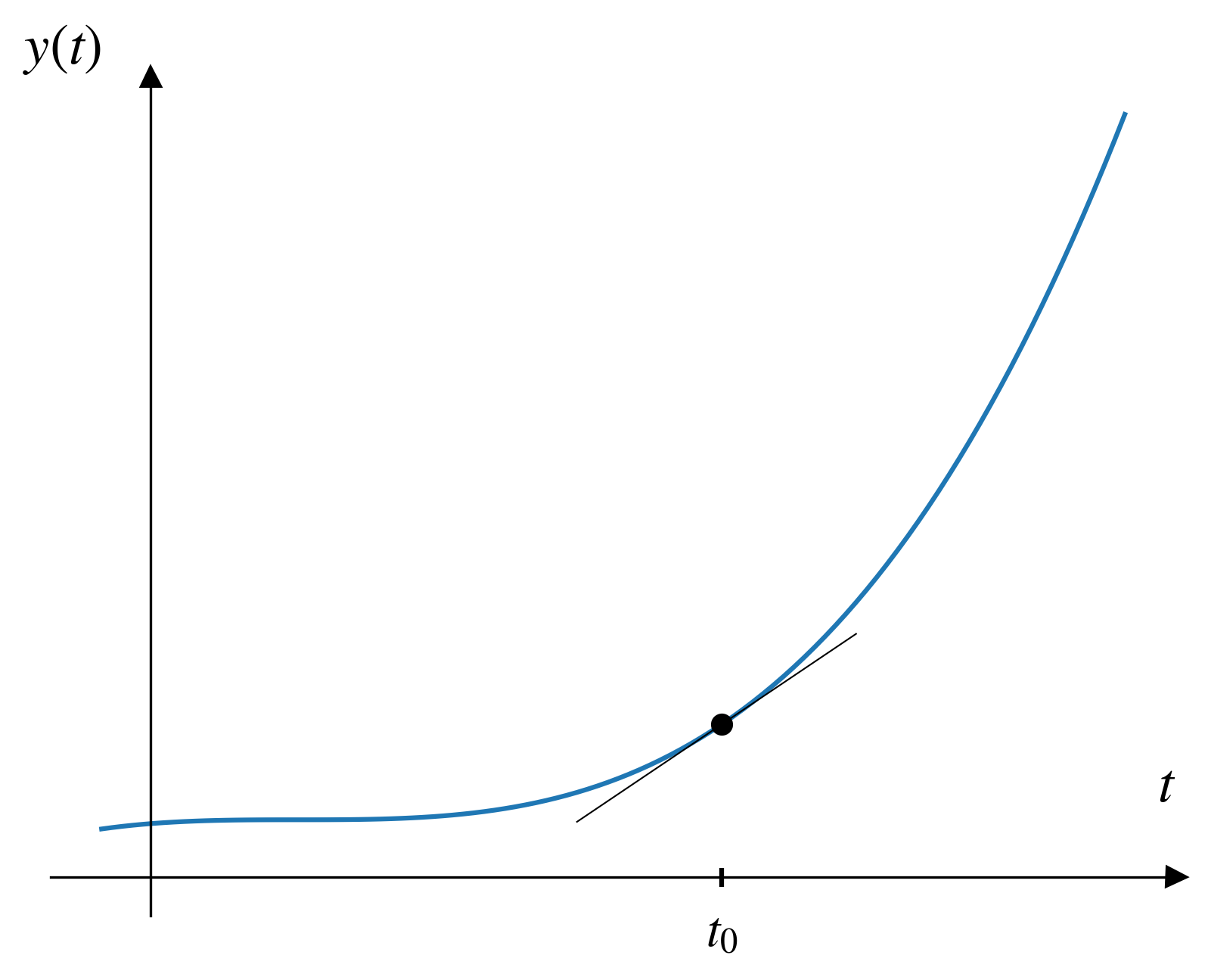
  1. I know the form of the differential equation (\(dy/dt = f(y,t)\))
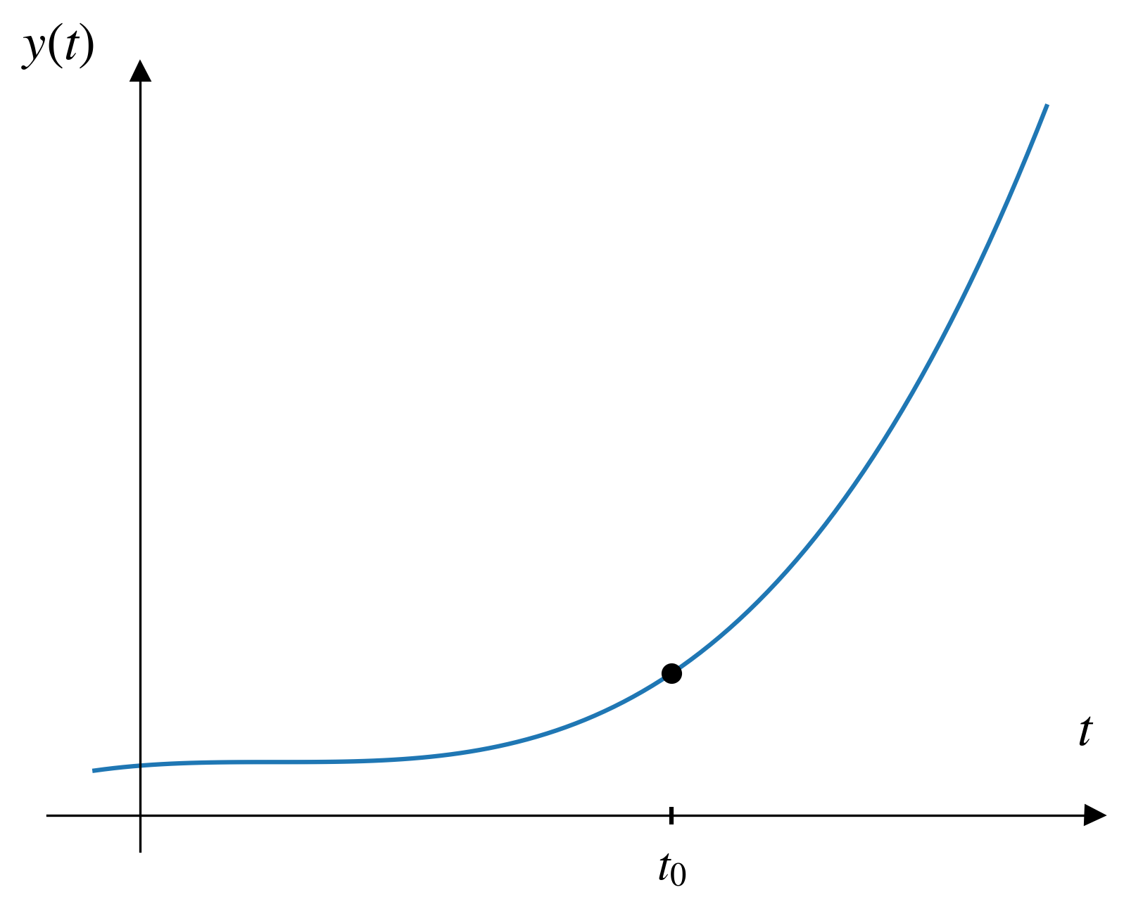
  2. I know the value at one point (initial condition)

Then..

  • I can estimate the value at some other time, very close to the known point.
  • And I can keep doing that to get as many points as I want.

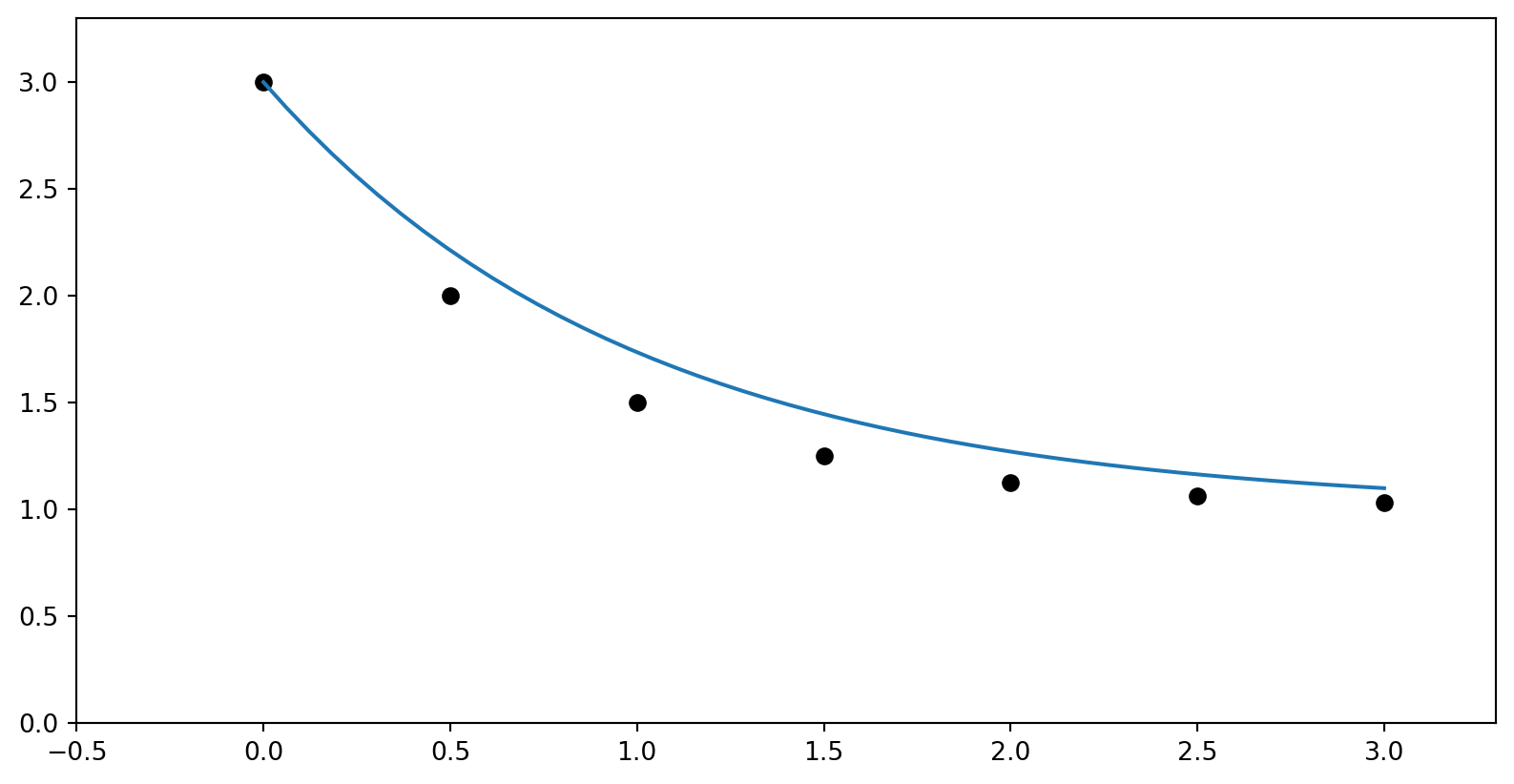
Visualizing Euler’s method

The key components

To solve a differential equation with Euler’s method we need to start with two things:

  1. A function describing the derivative of our parameter of interest
  2. An initial condition

Euler algorithm

Given:

  • A function for the derivative: \(f(t, y) = \frac{dy}{dt}\)
  • An initial condition: \(y(t_0) = y_0\)
  • Step size: \(\Delta t\)

For \(n = 1, 2, 3 \ldots\): \[t_{n+1} = t_n + \Delta t\] \[y_{n+1} = y_n + \Delta t \cdot f(t_n, y_n)\]

Example Problem

Use the differential equation and initial condition below to find \(y\) when \(t=2.5\):

\[y(t) = 1 - \frac{dy}{dt},\quad y(0) = 3\]

Let’s use Euler’s method with \(\Delta t = 0.5\) to approximate \(y(2.5)\).

Let’s rearrange the differential equation so we have a “function for the derivative”:

\[\frac{dy}{dt} = 1 - y(t)\]

Solution

Given:

\(y(0) = 3\)

\(\Delta t = 0.5\)

\(\frac{dy}{dt} = 1 - y(t)\)

Euler equations:

\(t_{n+1} = t_n + \Delta t\)

\(y_{n+1} = y_n + \Delta t \cdot \frac{dy}{dt}\)

n       t       y       dy/dt  
0       0.0     3.0     -2.0   
1       0.5     2.0     -1.0   
2       1.0     1.5     -0.5   
3       1.5     1.25    -0.25  
4       2.0     1.125   -0.125 
5       2.5     1.0625  -0.0625
y(2.5) is approximately 1.0625

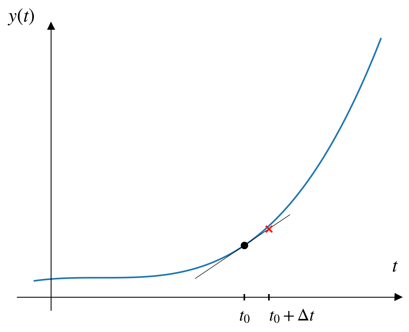
Visualizing the solution